Derivative Maps

I recently came across an interesting paper, Bump Mapping Unparametrized Surfaces on the GPU by Morten Mikkelsen of Naughty Dog. This paper describes an alternative method to normal mapping, closely related to bump mapping. The alluring prospect of this technique is that it doesn’t require that a tangent space be defined.

Mikkelsen is apparently well-versed in academic obfuscation (tsk!), so the paper itself can be a little hard to read. If you’re interested in reading it, then I would recommend first reading Jim Blinn’s original bump mapping paper to understand some of the derivations.

But Wait! What’s Wrong with Normal Maps?

Nothing really. But if something comes along that can improve quality, performance or memory consumption then it’s worth taking a a look.

A Quick Detour into Gradients

Given a scalar height field (i.e. a two-dimensional array of scalar values), the gradient of that field is a 2D vector field where each vector points in the direction of greatest change. The length of the vectors corresponds to the rate of change.

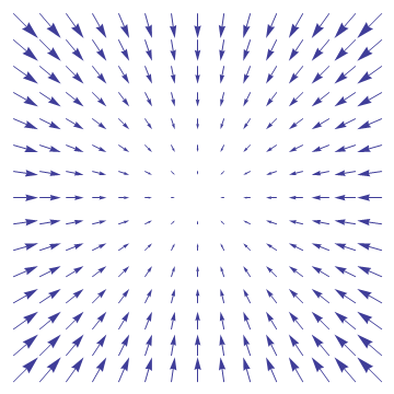
The contour map below represents the scalar field generated from the function . The vector field shows the gradient of that scalar field. Note how each vector points towards the center, and how the vectors in the center are smaller due to the lower rate of change.

Derivative Maps

The main premise of the paper is that we can project the gradient of the height field onto an underlying surface and use it to skew the surface normal to approximate the normal of the height-map surface. We can do all of this without requiring tangent vectors.

As with the original bump-mapping technique, it’s not exact due to some terms being dropped due to their relatively small influence, but it’s close.

There are really only two important formulae to consider from the paper. The first shows how to perturb the surface normal using the surface gradient. Don’t confuse the surface gradient with the gradient of the height field mentioned above! As you’ll see shortly, they’re different.

Here, represents the perturbed normal, is the underlying surface normal, and is the surface gradient. So basically, this says that the perturbed normal is the surface normal offset in the negative surface gradient direction.

So how do we calculate the surface gradient from the height field gradient? Well, there’s some fun math in there which I don’t want to repeat, but if you’re interested, I would recommend reading Blinn’s paper first, then Mikkelsen’s paper. You eventually arrive at:

In addition to the symbols defined previously, and are the partial derivatives of the surface position, and and are the partial derivatives of the height field. The derivative directions and are not explictly defined here.

It’s easiest to think of this as the projection of the 2D gradient onto a 3D surface along the normal. Intuitively, this says that the surface gradient direction is pushed out on orthogonal vectors to the s/n and t/n planes by however much the gradient specifies. The denominator term is there to scale up the result when the and are not orthogonal, or are flipped.

Implementation

Implementing this technique is fairly straightforward once you realise the meaning of some of the variables. Since we’re free to choose the partial derivative directions and , it’s convenient for the shader to use screen-space x and y. The value is the position, and the value is the height field sample.

// Project the surface gradient (dhdx, dhdy) onto the surface (n, dpdx, dpdy)
float3 CalculateSurfaceGradient(float3 n, float3 dpdx, float3 dpdy, float dhdx, float dhdy)
{
	float3 r1 = cross(dpdy, n);
	float3 r2 = cross(n, dpdx);

	return (r1 * dhdx + r2 * dhdy) / dot(dpdx, r1);
}

// Move the normal away from the surface normal in the opposite surface gradient direction
float3 PerturbNormal(float3 n, float3 dpdx, float3 dpdy, float dhdx, float dhdy)
{
	return normalize(normal - CalculateSurfaceGradient(normal, dpdx, dpdy, dhdx, dhdy));
}

So far, so good. Next we need to work out how to calculate the partial derivatives. The reason why we chose screen-space x and y to be our partial derivative directions is so that we can use the ddx and ddy shader instructions to generate the partial derivatives of both the position and the height.

Given a position and normal in the same coordinate-space, and a height map sample, calculating the final normal is straighforward:

// Calculate the surface normal using screen-space partial derivatives of the height field
float3 CalculateSurfaceNormal(float3 position, float3 normal, float height)
{
	float3 dpdx = ddx(position);
	float3 dpdy = ddy(position);

	float dhdx = ddx(height);
	float dhdy = ddy(height);

	return PerturbNormal(normal, dpdx, dpdy, dhdx, dhdy);
}

Note that in shader model 5.0, you can use ddx_fine/ddy_fine instead of ddx/ddy to get high-precision partial derivatives.

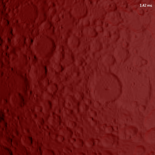
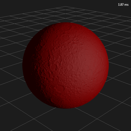
So how does this look? At a medium distance, I would say that it looks pretty good:

But what about up close?

Uh oh! What’s happening here? Well, there are a couple of problems…

The main problem is that the height texture is using bilinear filtering, so the gradient between any two texels is constant. This causes large blocks to become very obvious when up close. There are a couple of options for alleviating this somewhat.

One option is to use bicubic filtering. I haven’t tried it, but I would expect this to make a good difference. The problem is that it will incur an extra cost. Another option, suggested in the paper, is to add a detail bump texture on top. This helps quite a lot, but again it adds more cost.

In the image below I’ve just tiled the same texture at 10x frequency over the top. It would be better to apply some kind of noise function as in the original paper.

The second problem is more subtle. We’re getting some small block artifacts because of the way that the ddx and ddy shader instructions work. They take pairs of pixels in a pixel quad and subtract the relevant values to get the derivative. In the case of the height derivatives, we can alleviate this by performing the differencing ourselves with extra texture samples.

The first problem is pretty much a killer for me. I would rather not have to cover up a fundamental implementation issue with extra fudges and more cost.

What Now?

It’s unfortunate that this didn’t make it into the original paper, but Mikkelsen mentions in a blog post that you can increase the quality by using precomputed height derivatives. This method requires double the texture storage (or half the resolution) of the ddx/ddy method, but produces much better results.

You’re probably wondering how you can possibly precompute screen-space derivatives. We don’t actually have to. Instead we can use the chain rule to transform a partial derivative from one space to another. In our case we can transform our derivatives from uv-space to screen-space if we have the partial derivatives of the uvs in screen-space.

To calculate dhdx you need dhdu, dhdv, dudx and dvdx:

To calculate dhdy you need dhdu, dhdv, dudy and dvdy:

The hlsl for this is very simple:

float ApplyChainRule(float dhdu, float dhdv, float dud_, float dvd_)
{
	return dhdu * dud_ + dhdv * dvd_;
}

Assuming that we have a texture that stores the texel-space height derivatives, we can scale this up in the shader to uv-space by simply multiplying by the texture dimensions. We can then use the screen space uv derivatives and the chain rule to transform from dhdu/dhdv to dhdx/dhdy.

// Calculate the surface normal using the uv-space gradient (dhdu, dhdv)
float3 CalculateSurfaceNormal(float3 position, float3 normal, float2 gradient)
{
	float3 dpdx = ddx(position);
	float3 dpdy = ddy(position);

	float dhdx = ApplyChainRule(gradient.x, gradient.y, ddx(uv.x), ddx(uv.y));
	float dhdy = ApplyChainRule(gradient.x, gradient.y, ddy(uv.x), ddy(uv.y));

	return PerturbNormal(normal, dpdx, dpdy, dhdx, dhdy);
}

So how does this look? Well, it’s pretty much the same at medium distance.

But it’s way better up close, since we’re now interpolating the derivatives.

Conclusions

In order to really draw any conclusions about this technique, I’m going to need to compare the quality, performance and memory consumption to that of normal mapping. That’s a whole other blog post waiting to happen…

But in theory, the pros are:

• Less mesh memory: We don’t need to store a tangent vector, so this should translate into some pretty significant mesh memory savings.
• Fewer interpolators: We don’t need to pass the tangent vector from the vertex shader to the pixel shader, so this should be a performance gain.
• Possible less texture memory: At worst this method requires two channels in a texture. At best, a normal map takes up two channels.
• Easy scaling: It’s easy to change the height scale on the fly by scaling the height derivatives. This isn’t quite so easy to get right when using normal maps. See here. As Stephen Hill points out in the comments below, this is a pretty weak argument, so I’m removing it.

And the cons are:

• More ALU: It’s going to be interesting to see the actual numbers, but this is probably the only thing that could put the nail in the coffin for derivative maps. The extra cost for ALU might be compensated partially by the fewer interpolators, but we’ll have to see.
• Less flexible: A normal map can represent any derivative map, but the reverse is not true. I’m not sure that this is a significant problem in practice though.
• Worse quality? I’m not sure about this one, but it’ll be interesting to see if the quality holds up.